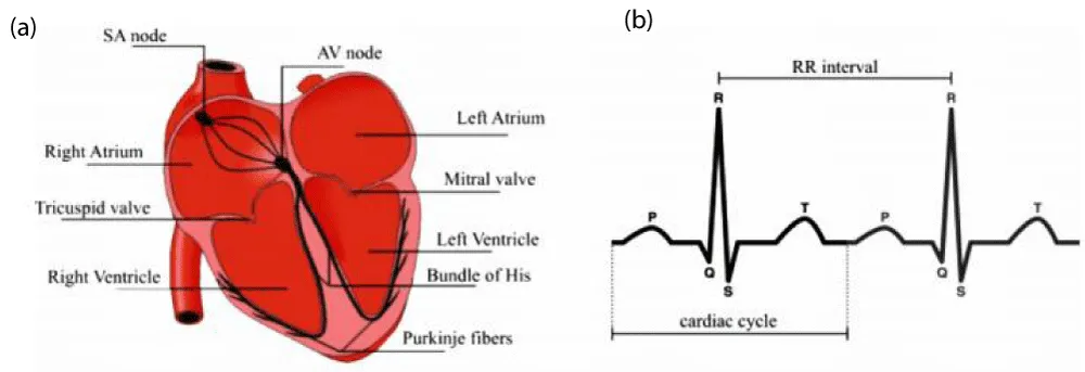
The regular and normal pumping of blood by the biological organs conditions the normal functioning of the heart [1-5]. Knowledge of cardiac activity is crucial in the analysis of the heart, as it can be regular or irregular in time and space [6,7]. Under certain conditions, this regularity or irregularity can reveal pathologies [8, 9]. These pathologies are identified by analysis of the cardiac system. The cardiac electrical system maintains its rhythm between 60 and 100 beats per minute. The functional diagram of the heart, with its main cardiac nodes representing the cardiac electrical conduction system, is shown in figure 1a. The normal response of a normal ECG, consisting of the main waves: the P wave, the QRS complex and the T wave, is shown in figure 1b.
Figure 1: Functional diagram of the electric system of conduction of the heart [10,11].
The cardiac system is made up of nodes ranging from the SA node, the AV node to the Purkinje fibers [12-15]. It functions like a pacemaker, so the precise point of electrical current creation is the sinus node, located at the apex of the right atrium. The electrical current is a few millivolts and is generated from a cluster of cells. From the sinus node, the current spreads like an oil slick through the heart muscle. It flows through the 2 atria to their base, causing them to contract. Then, through an electrical relay called the Atrioventricular Node (AVN), the electric current reaches the septum separating the atria and ventricles. Each electrical current path between the sinoatrial node and the ventricles causes a heartbeat. This sequence of electrical current flow from the sinus node to the Purkinje fibers is the origin of the electrocardiogram signal. The electrocardiogram records a succession of sequences of the heart's electrical activity, represented by P waves, the QRS complex and the T wave. The P wave is that of the atria at the moment of their contraction, the QRS complex corresponds to the contraction of the ventricles, and the T wave reflects the repolarization (return to the resting phase) of the ventricles. When the formation or conduction of electrical excitation is disrupted, we speak of arrhythmias [16-21].
In 1928, Van der Pol and Van der Mark proposed the first nonlinear oscillator model capable of modeling the pacemaker [22]. This oscillator is considered the starting point for cardiac modeling. Still with the aim of modeling heartbeats, a large number of pacemaker models have been proposed as nonlinear oscillators like Van der Pol. We note the works of Fonkou et al [23-27], FitzHugh [28] and Hodgkin-Huxley [29]. These oscillators present important characteristics, in particular their ability to undergo frequency entrainment phenomenon without altering their amplitudes, since the main pacemaker is the element of the conducting system with the highest frequency, to which all the other oscillators must adapt.
It should be noted that the study of the cardiac conduction system at the cellular level is not suited to this approach to heartbeat modeling, as it only enables an analysis of the heart rhythm to be made by studying the interactions between the various elements. In this option, based mainly on the interactions between cardiac nodes, numerous works have been done focusing mainly on the interaction between AV, SA nodes and Purkinje His bundles. Among these works, we note in 2009 the work of Gois and Savi [30]. They model the cardiac system as a set of three Grudzinski-Zebrowski oscillators coupled unidirectionally to each other by delayed connections. In 2022, Fonkou et al [31] also proposed a model of the heart as an ensemble of three FitzHugh-Nagumo-type oscillators coupled by delayed connections. In 2021, Cheffer et al improved on the model proposed by Gois and Savi [32]. In the same context, random connections have been studied [33-35]. In 2023 Fonkou and Savi improved the heart system by proposing a reduced-order model to describe different heart rhythms by incorporating delayed Duffing-type connections. They also described variations in sinus rhythm by a time-dependent frequency, representing transient disturbances [36]. We also note the work of Krstacic et al [37], Ernst and Bar-Joseph [38], Tobon et al [39].
However, a large number of external and physiological constraints can affect cardiac activity, leading to the appearance of life-threatening pathologies requiring a controller in these situations. Among these controllers we can mention artificial pacemakers and implantable heart defibrillators. The latter are devices capable of impacting heart rhythm management, as they are for the most part powered by batteries that need to be replaced or recharged after a period of operation. They must therefore be monitored by appropriate controllers linked to probes that monitor heart activity or body response [40]. In recent years, the concept of monitoring has emerged as a plausible way of optimizing and automating biological assist devices, including artificial pacemakers [40,41].
In this context, a large number of approaches to heart rate control have been developed [42-44]. These include the classic method of Garfinkel et al [42, 45], and the work of Ferreira et al [46], in which they control the dynamics of a pacemaker using feedback control. In 2014, they proposed a more general analysis for ECG control [47], which stabilizes unstable periodic orbits embedded in chaotic attractors allowing critical physiological situations to be managed. In 2020, Lounis et al [44] developed a highorder control method to solve the dynamic problems of the model proposed by Quiroz-Juarez et al [48]. In 2020, an active control based on the Lyapunov method was proposed by Khan and Nigar [49]. Faced with the difficulty of solving all the non-linearity problems inherent in systems, such as approximation errors and external disturbances, some control methods appear to be ineffective. Some researchers have tried to solve them using the state observer method [50]. This method has not been satisfactory because it is limited. Others, however, have used machine learning incorporating artificial neural networks (ANNs) [51-53]. This method has proved highly effective. For example, in 2023, Lima et al., [41] developed an intelligent control method using artificial neural networks to eliminate heart rhythm problems. In their work, they evaluate the ability of the control law to manage intra- and inter-patient variability by considering the control variable at the level of the His-Purkinje complex. Machine learning, for its part, may offer attractive options for dealing with this. Artificial neural networks (ANNs), for example, have been used to identify and classify heart rhythm diseases [51-53]. Because of their learning and approximation capabilities, neural networks have also been used in control applications to compensate for model uncertainties and perturbations [54-57].
In this article, considering the reduced-order model developed by Fonkou and Savi [36], consisting of three non-linear oscillators linked by delayed Duffing-type connections, a test for the control of heart rhythm is carried out. In order to have an overall idea of the behavior of the model, an analysis of its stability in its autonomous, unidirectionally coupled state is carried out. It reveals regions of stable and unstable periodicities describing very rich dynamic behaviors. Since the electrical signal responsible for powering the heart's organs is generated by the SA node, a disturbance of the heart rhythm is caused at the SA node, leading to the appearance of cardiac pathologies such as ventricular fibrillation, ventricular flutter, atrial fibrillation and atrial flutter. To manage this, a control strategy has been developed. It consists in following the signal trajectories of the sinus node. For better compensation of unknown or hidden heart dynamics, the feedback linearization method (FBL) is used numerically, integrating Artificial Neural Networks (ANNs) to compensate for unknown dynamics. The observed dynamic is the electrocardiogram (ECG) signal. Based on synthetic ECGs, the results obtained show that FBL enables the heart to maintain its normal rhythm, avoiding pathological rhythms. In order to also achieve a real-life implementation of the model used, an electronic simulation of the heart system was carried out using OrCAD-PSpice software. The results obtained show good agreement with those obtained numerically.
The rest of the work is organized as follows: the mathematical modeling of the heart model is presented in section 2. System stability is analyzed in session 3. It shows regions of stable and unstable periodicities describing very rich dynamics. Section 4 presents the normal dynamics of the synthetic ECG. Pathological ECGs are highlighted in section 5. The details of the controller are developed in section 6. Section 7 shows the impact of control on the system. Results obtained by electronic simulation on OrCAD-PSpice are given in section 8. The work ends with a conclusion in section 9.
Mathematical modelling
As is well known, two pumps - the left and right ventricles - are essential parts of the heart. They are contracted by the electrical impulse produced by the heart through its electrical system, known as the electrical conduction system of the heart. Its role is to ensure a regular heartbeat. For good functioning of the electrical conduction system, the amount of blood needed to oxygenate the lungs is pumped by the right ventricle, and the amount of blood needed to oxygenate the whole body is pumped by the left ventricle. This analysis shows that the greatest mechanical work is done by the left ventricle. All this is due to the regularity of the cardiac conduction system It is composed of the sinus node, the atrioventricular node and Purkinje's His bundles. The electrical impulse which causes the contraction of the atria and ventricles is initiated by the sinus node (the heart's natural pacemaker). After receiving information from the brain, the SA node adapts the heart rate in accordance with the body's energy requirements. In its normal state, heart rate varies between 1 and 1.67 Hz. The electrical impulse initiated by the SA node enables the blood to reach the ventricles after having passed through the two auricles by contracting them. The atrioventricular node in turn receives this electricity, filters it, slowing it down, if necessary, in cases of rhythm disorders, and then directs it through Purkinje's His bundles to the ventricles, also enabling the ventricles to contract. This is how electricity travels through the heart. Each heartbeat forming the electrocardiogram (ECG) signal is caused by each electrical current pathway from the sinus node to the ventricles.
Recent work has shown that heartbeat modeling is a crucial process for the automatic identification of characteristic waves [10,11]. The objective is to propose the simplest, most compact mathematical model capable of qualitatively and quantitatively simulating the shape of the five main waves (P,Q,R,S and T waves) constitutive of heartbeats. Indeed, the most natural representation of the waves would be to describe the signal by its amplitude at each instant; this representation would therefore be a vector in a space whose dimension would be equal to a few hundred. From these analyses, cardiac physiology has been modeled as a system of three oscillators subjected to external stimuli and coupled together by delayed connections [36]. These stimuli have the effect of increasing the dimension of the reduced-order model system and also represent spatio-temporal stimuli.
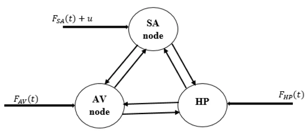
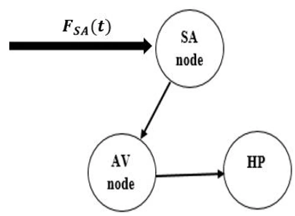
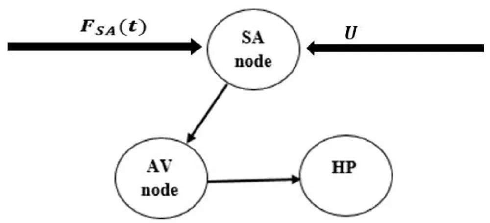
In this subsection, the mathematical model is that proposed by Fonkou and Savi [36]. This is a system of three nonlinear oscillators coupled by delayed Duffing-type connections incorporating cubic non-linear terms. These three oscillators consist of the SA node, the AV node and the Purkinje fibers linked by Duffing-type connections with delay and non-delay. For this work, in addition to the external stimuli to which each oscillator is subjected, the SA oscillator is subjected to the controller u as presented by its conceptual model of general functioning given in figure 2. The mathematical model describing them is given by equation (1).
Figure 2: Conceptual model of general functioning of the heart with controller.
Where u is the controller. The SA, AV and HP nodes are described respectively by the pairs
. Coefficients between two nodes m and
without delay and with delay are given by
and
(m and n can express the SA, AV or HP node as well). The linear and cubic terms with delay are:
and
, and those without delay are
and
is the external excitation making the system temporarily dependent and increasing its dimension.
is the transient frequency disturbing the SA node. It is a function of time and is described by
is the transitional phase between
and
the transition time. In this work its influence will be neglected, it will take the values
Using a combination of three nodes (SA, AV and HP), the mathematical expression of the ECG signal is given by
With
Where
and
are constant parameters. In addition, it is possible to write:
Considering the equations of the system (1) adimensioned, the parameters to conform with them are given by:
where
. It can also be considered as the ratio between the experimental value and the numerical value
. Here the external excitations are considered as harmonics:
and
. All simulations consider
and
, for all the simulations, we will take as initial conditions :
and
.
Note that the model parameters are estimated from the same real ECG data and can be either deterministic or non-deterministic. In deterministic situations, each rhythm is considered to be associated with a set of parameters, and a change in that rhythm is attributed to a change in those parameters. In other words, a pathological rhythm can be understood as resulting from a change in these parameters. In contrast, nondeterministic situations involve random variations in the parameters that can lead to pathological rhythms. t should also be noted that the constants of the coupled Duffing model are physiologically grounded: the natural frequencies
reproduce the intrinsic automaticity of the SA node ( 1 Hz ), the AV node ( 0.7 Hz ), and the His-Purkinje system (0.4" " Hz) [58]. The delays τi correspond to the PR interval of 0.1 s and the QRS interval of 0.08 s measured on a 12 -lead ECG [59]. The coupling coefficients
model the conductances of connexin-mediated junctions, the reduction of which explains AV block [60]. The Duffing nonlinearities αi and
and
are justified by the nonlinear current-voltage relationship of the voltage-dependent
channels [28]. The synthetic ECG generated is therefore the weighted sum of the three oscillators, in accordance with the principle of superposition of cardiac dipoles [61].
It should also be noted that changing the value of a constant alters the nature of the ECG signal in accordance with the clinical case. For example, a decrease in one of the
values can lead to a prolongation of the PR interval, which would imply the onset of AV block. An increase or decrease in
can alter the T wave and, in some cases, lead to hyperkalemia.
All of these analyses were presented in the manuscript, and the parameter changes were provided in Table 2 of the manuscript, yielding the curves shown in Figures 7-10.
This transforms the mathematical model into a physiological model. Furthermore, considering the equation for a cardiac oscillator given by:
modifies the shape of the pulse, resulting in a change in the refractory period. ei Controls the diastolic period; the self-oscillatory nature is maintained whenr
. Varying
and
allows the resting potential to be lowered or raised, which decreases or increases the frequency of action potential generation. This occurs without affecting the amplitude of the oscillations [62]
is the external stimulus that originates from a spatiotemporal stimulus and is therefore considered a reduced-order representation of spatiotemporal aspects
Fixed points analysis
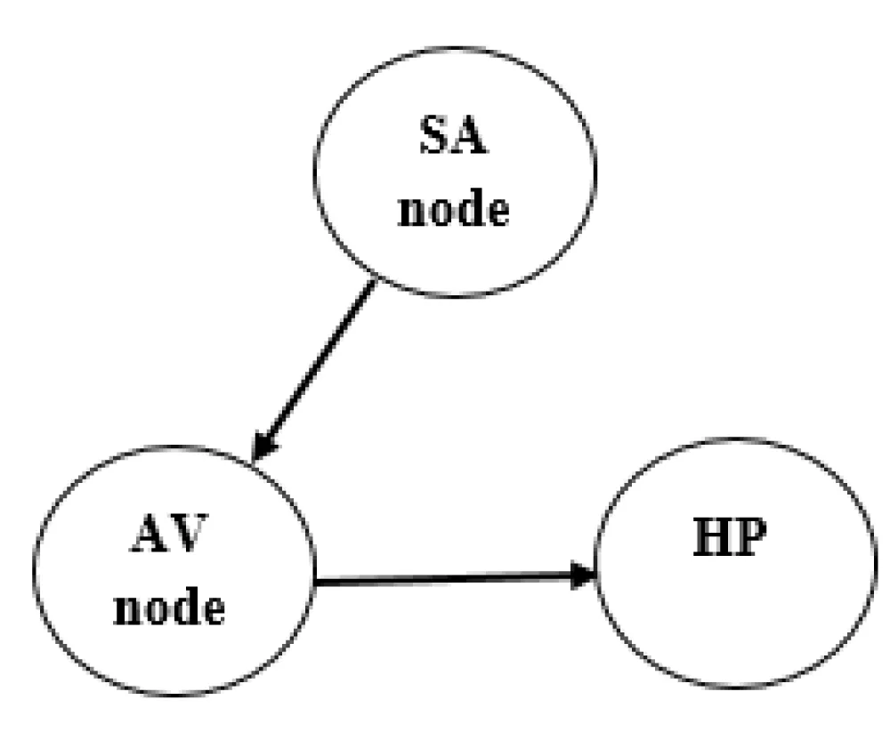
The search and analysis of equilibrium points is carried out by considering the model in its unidirectional connection state. In this case, its conceptual model is given in figure 3, the mathematical model characterizing it is given by equation (6) and the parameters for obtaining normal dynamics in Table 1, Figure 3.
| Table 1: Heart system parameters for ECG simulation. |
| Coupling parameters |
SA Oscillator |
AV Oscillator |
HP Oscillator |
parameter |
|
|
|
|
|
|
|
|
|
|
|
|
|
|
|
|
|
|
|
|
|
|
|
|
|
|
|
|
|
|
|
|
|
|
|
|
Figure 3: Conceptual model of normal functioning of the heart.
Fixed points
The fixed points or equilibrium points of this system are obtained by solving the system (7).
(7) To facilitate the search for fixed points, a Taylor expansion [63] is proposed. The delay terms make the system more complex, but this allows for more manageable equations. This expression is given in equation (8) and the new system in equation (9).
With
A detailed, step-by-step derivation of equations (9) and (10) is provided in Appendix A Using Cardran's solution method [64], we obtain 27 equilibrium points, 5 of which are actual equilibrium points, namely:
complex equilibrium points, namely:
The stability analysis is made by computing the Jacobean matrix of the system (6). This matrix is given by equation (11).
With
The verification of the Jacobian matrix reductions is provided in Appendix B. By resolving
, we obtain the characteristic equation (13).
Using the Ruth-Hurwitz stability criterion, equation (13) gives us 4 stable fixed points and 23 unstable fixed points. The stable fixed points are:
et
and
are asymptotically stable,
and
are marginally stable.
For the fixed point
, we have the following eigenvalues:
For the fixed point
, we have the following eigenvalues:
0.0002i
For the case of a fixed point
, the eigenvalues are:
0.0002i
On the other hand, the fixed point
, we have the following eigenvalues:
Normal synthetic ECG
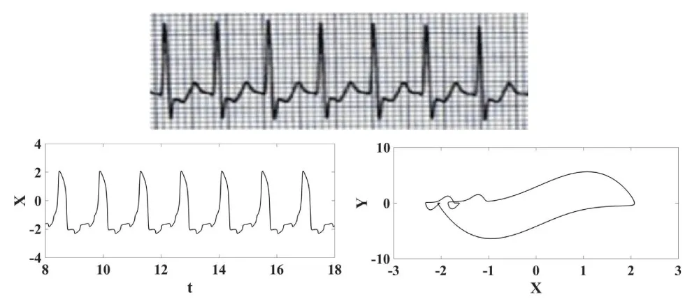
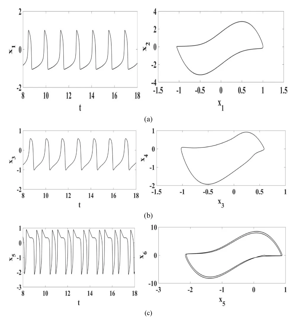
Considering the synthetic model of heart function (Figure 3) and the parameters for obtaining normal rhythms given in Table 1, the synthetic ECG is observed in Figure 4.
Figure 4 shows the synthetic ECG signal obtained by digital simulation. The presence of the five main ECG waves is observed, namely the P waves, the QRS complex and the T wave. A comparison with a signal recovered from a real recording is made [65]. The different dynamics of the SA, AV and HP nodes are given in Figure 5.
Figure 4: Normal ECG. (a) Experimental recorded ECG signal [60] (b) Synthetic ECG time series; (c) Synthetic ECG state space.
Figure 5: Normal synthetic ECG represented by each one of the oscillator responses in the form of time series and state space. (a) SA node; (b) AV node; (c) HP complex.
Pathological synthetic ECGs
In this section, the presentation of cardiac pathologies obtained when only the sinus node is disturbed in the absence of any control signal (u = 0) is described following the mathematical model. None of the parameters of the main system in its normal state are modified. Only external stimulus parameters related to the sinus node are modified. In this case, the system is disturbed only at the level of its sinus node and the other disturbances are not considered since we only wanted to control the heart by following the trajectory of the SA node. According to the values taken by the parameters
and
, four types of pathologies dangerous for the normal functioning of the heart are highlighted in order to observe the power of our controller. These are ventricular flutter, ventricular fibrillation, atrial fibrillation and atrial flutter. Their conceptual model is given in Figure (6) and the parameters of obtaining these different pathologies are in table 2,
Figure 6: Conceptual model of heart functioning in its pathological state.
| Table 2: Heart system parameters for simulation of cardiac pathologies. |
| SA Oscillator |
AV Oscillator |
HP Oscillator |
Forcing Terms |
Coupling Terms |
ECG Parameters |
| Ventricular Flutter |
|
|
|
|
|
| αSA = 14.0 |
αAV = 12.0 |
αHP = 12.0 |
ρSA = 35.6 |
kSA–AV = 1.2 |
a₁ = 2.0 |
| vSA₁ = 0.52 |
vAV₁ = 0.01 |
vHP₁ = 0.1 |
ωSA = 6.94 |
kAV–HP = 1.1 |
a₂ = 0.01 |
| vSA₂ = −0.5 |
vAV₂ = −0.4 |
vHP₂ = −1.4 |
ρAV = 0.0 |
kτSA–AV = 1.1 |
a₃ = 0.15 |
| dSA = 2.0 |
dAV = 3.0 |
dHP = 7.0 |
ωAV = 0.0 |
kτAV–HP = 1.1 |
aτ = 1.0 |
| eSA = 3.0 |
eAV = 5.91 |
eHP = 1.0 |
ρHP = 0.0 |
τSA–AV = 0.8 |
|
| |
|
|
ωHP = 0.0 |
τAV–HP = 0.1 |
|
| Atrial Fibrillation |
|
|
|
|
|
| αSA = 14.0 |
αAV = 12.0 |
αHP = 12.0 |
ρSA = 1.6 |
kSA–AV = 1.2 |
a₁ = 2.0 |
| vSA₁ = 0.52 |
vAV₁ = 0.01 |
vHP₁ = 0.1 |
ωSA = 1.94 |
kAV–HP = 1.1 |
a₂ = 0.01 |
| vSA₂ = −0.5 |
vAV₂ = −0.4 |
vHP₂ = −1.4 |
ρAV = 0.0 |
kτSA–AV = 1.1 |
a₃ = 0.15 |
| dSA = 2.0 |
dAV = 3.0 |
dHP = 7.0 |
ωAV = 0.0 |
kτAV–HP = 1.2 |
aτ = 1.0 |
| eSA = 3.0 |
eAV = 5.91 |
eHP = 1.0 |
ρHP = 0.0 |
τSA–AV = 0.8 |
|
| |
|
|
ωHP = 0.0 |
τAV–HP = 0.1 |
|
| Atrial Flutter |
|
|
|
|
|
| αSA = 14.0 |
αAV = 12.0 |
αHP = 12.0 |
ρSA = 0.66 |
kSA–AV = 1.2 |
a₁ = 2.0 |
| vSA₁ = 0.52 |
vAV₁ = 0.01 |
vHP₁ = 0.1 |
ωSA = 0.35 |
kAV–HP = 1.1 |
a₂ = 0.01 |
| vSA₂ = −0.5 |
vAV₂ = −0.4 |
vHP₂ = −1.4 |
ρAV = 0.0 |
kτSA–AV = 1.1 |
a₃ = 0.15 |
| dSA = 2.0 |
dAV = 3.0 |
dHP = 7.0 |
ωAV = 0.0 |
kτAV–HP = 1.2 |
aτ = 1.0 |
| eSA = 3.0 |
eAV = 5.91 |
eHP = 1.0 |
ρHP = 0.0 |
τSA–AV = 0.8 |
|
| |
|
|
ωHP = 0.0 |
τAV–HP = 0.1 |
|
| Ventricular Fibrillation |
|
|
|
|
|
| αSA = 14.0 |
αAV = 12.0 |
αHP = 12.0 |
ρSA = 30.6 |
kSA–AV = 1.2 |
a₁ = 2.0 |
| vSA₁ = 0.52 |
vAV₁ = 0.01 |
vHP₁ = 0.1 |
ωSA = 6.99 |
kAV–HP = 1.1 |
a₂ = 0.01 |
| vSA₂ = −0.5 |
vAV₂ = −0.4 |
vHP₂ = −1.4 |
ρAV = 0.0 |
kτSA–AV = 1.1 |
a₃ = 0.15 |
| dSA = 2.0 |
dAV = 3.0 |
dHP = 7.0 |
ωAV = 0.0 |
kτAV–HP = 1.2 |
aτ = 1.0 |
| eSA = 3.0 |
eAV = 5.91 |
eHP = 1.0 |
ρHP = 0.0 |
τSA–AV = 0.8 |
|
| |
|
|
ωHP = 0.0 |
τAV–HP = 0.1 |
|
Case of ventricular flutter
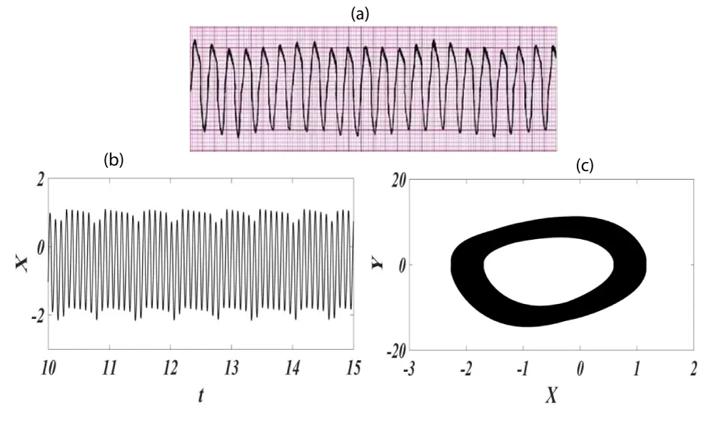
Ventricular flutter is a highly intolerable arrhythmia. In this arrhythmia, the ECG shows an equalsized undulation of the QRS complexes, with no isoelectric line between them and no T wave. There is no evidence of any separation between the QRS and the ST-T. During the onset of ventricular flutter, a high heart rate of between 250 and 300/min is noted. As in the case of ventricular fibrillation, an emergency response is required to avoid recurrence, and a therapeutic approach is necessary. Although it can occur spontaneously, supraventricular tachycardia (SVT) is usually the cause of a heart attack.
It is also manifested by a regular appearance of the cardiac rhythm, absence of the P wave, no true QRS complexes, they are widened (> 0.10 seconds) and of sinusoidal shape, a ratio P wave complex QRS not measurable, a PR interval also not measurable [66]. The presence of influx formation due to an ectopic focus on the left and right branches of the His bundle or the Purkinje network (tertiary automatism center) is also observed. In addition, we also note incessant re-entry of the influx at the level of the branches and network of Purkinje or sometimes in the myocardial fibers.
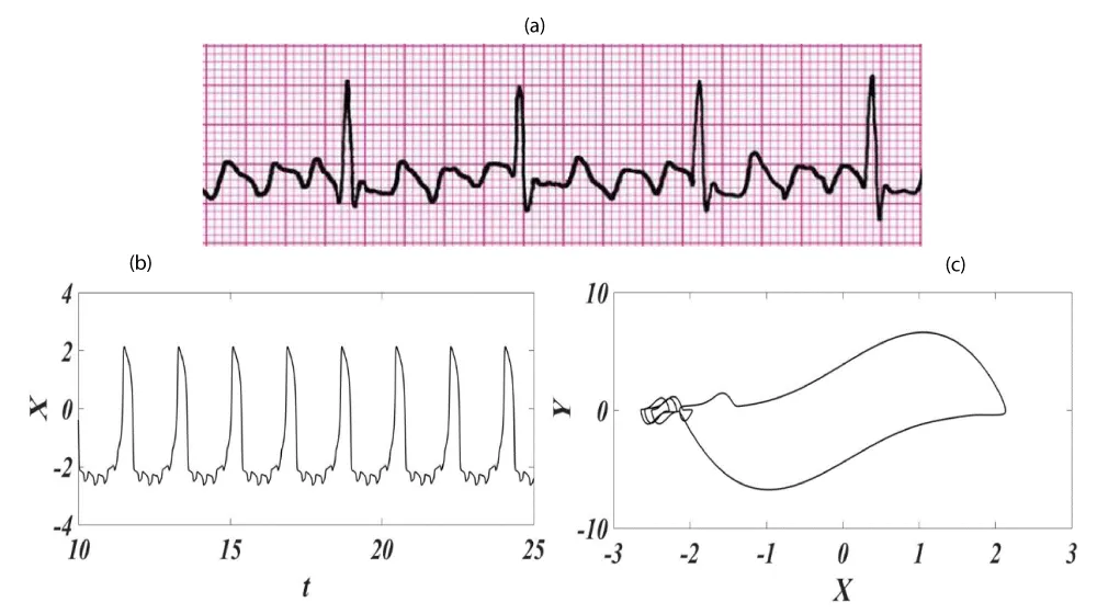
The dynamics of the ECG are given in Figure 7. Figure 7b shows the time series and Figure 7c the state space. The signal of an ECG obtained from a real recording is shown in Figure 7a [67]. It allows a qualitative comparison with the digitally obtained ECG (Figure 7b).
Figure 7: Ventricular flutter ECG signal. (a) Recorded experimental ECG signal [67]; (b) Synthetic ECG time series; (c) Synthetic ECG state space.
Case of atrial fibrillation
This is a cardiac arrhythmia characterized by irregular heartbeats due to abnormal acceleration of the heart caused by rhythm disorders [68]. Old age is also a factor favoring the onset of this arrhythmia. The presence of cardiac pathology (hypertension, heart valve disease, etc.), obesity, or obstructive sleep apnea syndrome is also noted. When atrial fibrillation occurs, the atria are the focus of frequent, ineffective electrical impulses, which can lead to:
- very rapid, jerky contractions (400 to 600 beats / minute) of the atria, resulting in immobility of this part of the heart.
- Poor contraction of the atria due to blood stagnation. This is the risk of a cerebral vascular accident due to the propulsion of clots or thrombus in the artery.
- Rapid, irregular beating of the ventricles at around 150 beats per minute (known as tachyarrhythmia) caused by accelerated contraction of the ventricles, located below the atria. Heart failure can occur.
Arrhythmia can also occur in episodes lasting several days, between which a regular heartbeat is observed. It can also be permanent (in which case the irregularity of cardiac contractions is constant).
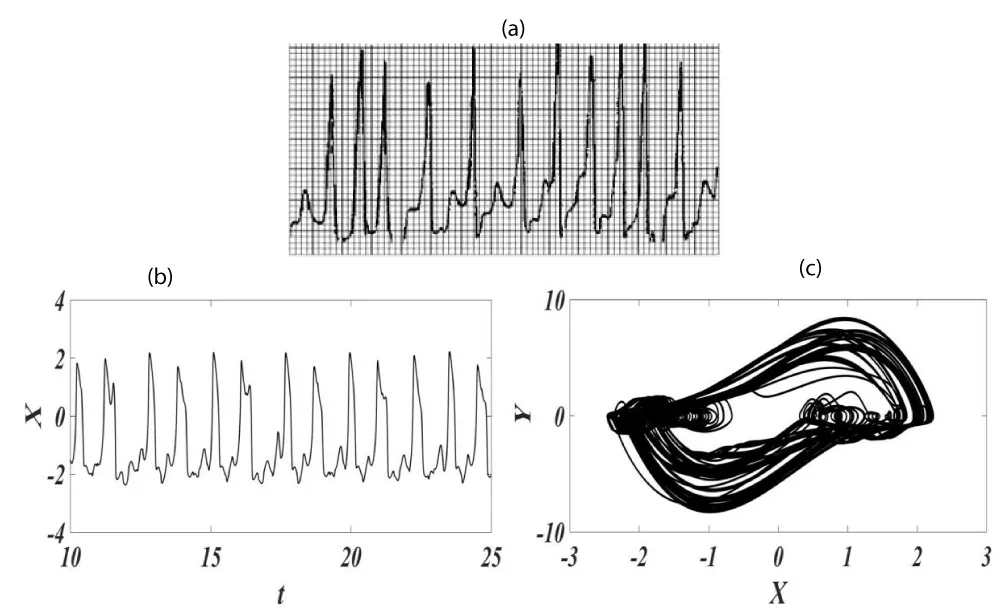
The ECG dynamics are given in Figure 8. The real ECG recording is observed in figure 8a [67], the time series and the state space of the ECG obtained digitally in figures 8b and 8c. A qualitative comparison is made between Figures 8a and 8b.
Figure 8: Atrial fibrillation ECG signal. (a) Recorded experimental ECG signal [67]; (b) Synthetic ECG time series. (c) Synthetic ECG state space.
Case of atrial flutter
This is a cardiac arrhythmia marked by the presence of a regular rapid rhythm secondary to a macrocircuit of intra-atrial reentry [69]. When palpitations and sometimes asthenia, exertional intolerance, dyspnea, and presyncope are present, these are referred to as symptoms of atrial fibrillation. An ECG helps to better diagnose the condition. This arrhythmia affects people above the age of 60. It accounts for some 60-65% of adult atrial tachycardias (excluding atrial fibrillation). Approximately 1% of people over 80 account for the number of cases of atrial fibrillation.
In the right atrium, there is a macroreentry circuit. Depolarization of the atria is also observed, with a rate of 250 to 300/min (usually 300/min). This frequency does not affect the AV node, and the ventricles are affected by every other atrial activation (2:1 block), inducing a regular ventricular frequency of 150 beats/minute. Occasionally, in AV block, an irregular ventricular rhythm is observed due to beat-to-beat variation. A fixed 3:1, 4:1 or 5:1 block may also be present, although this is generally less frequent.
By medication, prevention of thrombo-embolic events by anticoagulants, etc., the heart rate can be controlled.
For this case, Figure 9 shows the ECG dynamics: Figure 9a we have the ECG signal obtained from a real recording [67], Figure 9b the time series and Figure 9c the state space obtained digitally. A qualitative comparison is made between the digital ECG and the recorded ECG.
Figure 9: Atrial flutter ECG signal. (a) Recorded experimental ECG signal [67]; (b) Synthetic ECG time series. (c) Synthetic ECG state space.
Case of ventricular fibrillation
Considered the most severe arrhythmia, ventricular fibrillation is an uncoordinated, potentially lethal series of very rapid, ineffective contractions of the ventricles (lower chambers of the heart), caused by numerous chaotic electrical impulses [70]. In such arrhythmias, one observes very weak or absence of contraction on the part of the ventricles, resulting in very rapid, asynchronous pulsations. One of the consequences is cardiac arrest due to the complete cessation of blood flow. The heart frequency is constantly above 300, with discrete QRS complexes on the electrocardiogram.
Age is an important factor in the development of ventricular fibrillation. Other factors can also be a cause of ventricular fibrillation, including diabetes, hypertension, and underlying heart disease. Major consequences include heart failure and CVA.
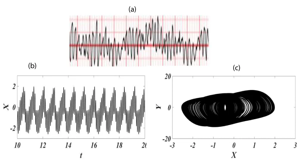
For this case, Figure 10 shows the ECG dynamics: Figure 10a present the ECG signal obtained from a real recording [67], Figure 10b the time series and Figure 10c the state space obtained digitally. A qualitative comparison is made between the digital ECG and the recorded ECG.
Figure 10: Ventricular fibrillation ECG signal. (a) Recorded experimental ECG signal [67]; (b) Synthetic ECG time series; (c) Synthetic ECG state space.
Controller
Recent work on control strategies shows a wide variety of intelligent control systems, used in the control of chaotic systems [71,72], robotic systems [73], under-actuated systems [69], also for the control of unexpected dynamics in non-linear systems [74]. In cardiac systems, their particularity lies in their ability to pick up cardiac signals, analyze them and then ask the controller to act [41]. In order to prevent the heart from being blocked, the systems used as controllers do not apply permanent control. They act only when they observe an abnormal rhythm, and then cease to act once the heart has returned to its normal operating state.
In order to return the heart to its normal functioning state when confronted with external disturbances that could lead it to a pathological operating state, an intelligent controller is implemented. It consists in tracking the trajectory of the SA node signals (in order to stabilize the ECG), the general operation depending only on the state to be controlled and its derivatives (generally the first derivative), and the calculation of the tracking error. The mathematical expression of this controller is given below by equation (14):
With u the control signal likely to act on the sinus node in the event of an abnormal heart functioning. The vector field part of the system (1) is represented by g. The hidden dynamics and other specifics of the heart rhythm are represented by p. The controlled states are (
). Using the feedback linearization method [41], the control signal obtained by a combination of feedback errors, desired states, and estimation of the unknown dynamics is given by:
Where
and p_ est are the estimates of g,b and p respectively, the feedback error is
, its first derivative is
is the desired state of the sinus node, and being the control parameter. Replacing u by its expression in equation (14) gives
Equation (16) is obtained by considering all modeling uncertainties are correctly represented by ρ, and also assuming that
is the approximation error.
Using the principle of the sliding mode method, the linear combination of feedback errors is given by
It is found that if s = 0, a first-order differential equation whose states
and
will converge to zero with a speed co-controlled by λ is obtained, i.e. the more lambda increases, the more the feedback errors converge to zero. From equation (17), the closed-loop dynamics (Equation (16)) becomes:
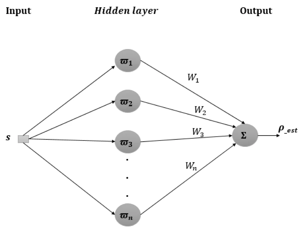
It is known that any approximation can be performed using radial basis function (RBF) networks. Using the desired degree of accuracy, an approximation of p is given by
, with
optimal estimation and
Thus, the calculation of uncertainty and estimated unmodeled dynamics is done using the RBF in Figure 11. Its expression is:
Figure 11: Radial basis function network with one input, n neurons in the hidden layer and one output.
Where
is the weight vector and
represents the vector of activation functions
being the number of neurons in the hidden layer. The dot function calculates uncertainty and estimated unmodeled dynamics: an internal product of the weight neural network and the activation function
The activation function at each neuron in the neural network is similar to a Gaussian distribution and given by the equation (19)
Where
and
respectively represent the centers and widths of the activation function. By applying s to the input, the order of complexity of the neural network is reduced and made sufficiently flexible, which allows it to be easily inserted into intelligent systems for cardiac rhythm control. A study of the bounding and convergence of the s and W signals is carried out using Lyapunov-type stability. For this purpose, a difference between the actual weight vector and the optimal weight vector, respectively, W and W+ is define by
Knowing that
, with
, and
. Thus equation (18) takes the form :
From equation (20), we obtain the differential equation (21) given by:
Equation (21) confirms the influence of approximation errors on the dynamic behavior of the system when operating in a closed loop. Hence the interest in integrating a neural network capable of making a universal estimate [71] for which the weights can be known on-line.
Suppose a positive function U defined by the equation (22)
Where µ is the learning rate. For µ = 0, neural network learning is disabled and only the FBL scheme is applied. For
and
. For
and
Assuming
ste,
and U is given by:
W for
, we have:
From equation (23) it can be seen that W is only limited for
. Using the projection algorithm studied in [72], the limit problem of is guaranteed and its domain of definition is taken equal to
Where
is the desired upper limit. It is used to control the limit of increase of the weight neural network. So any value of. So any value of
, it will always be less than
, hence
, which implies
. By replacing s by its expression taken from equation (9), we obtain equation
The multiplication of equation (25) by
gives the equation
By integrating (26) between 0 and t and multiplying the result
, we obtain
For
equation (27) results in
Inserting (28) into (25) gives :
Equation (29) leads to the conclusion that the exponential convergence of the tracking error to the closed region
et
is guaranteed by the controller.
Controlled dynamics
In this section, the results obtained digitally after implementation of the control are presented. The sampling frequency of the signals obtained is taken to be 100 Hz. To obtain the numerical results, the controller is programmed to follow the disturbed trajectories of the SA node, since in its disturbed state, the heart operates in pathological behavior (Figure 5). To normalize the system, a text file with the desired SA node signals extracted from a normal rhythm (from previous simulations) is read in. Since the sinus node is the seat of the electrical impulse, because it takes information from the brain and adapts the heart rate according to the body's needs, the electrical impulse from the sinus node will in turn travel through the two atria, contracting them and encouraging the passage of blood to the ventricles. The electrical impulse then reaches the AV node, where it is filtered and slowed down in the event of disruption of the SA node, before reaching the ventricles. The electrical impulse reaching the ventricles contracts them, enabling the right ventricle to propel blood to the lungs and the left ventricle to the rest of the body. By disrupting the sinus node, the course and nature of the electrical impulse through the heart is also disrupted, resulting in cardiac arrhythmias in the heart. In the present case, the pathological rhythms revealed are: ventricular flutter, ventricular fibrillation, atrial flutter or atrial fibrillation.
The learning rate and control parameter are
and
respectively. Taking
0, it is assumed that the control system is known without any knowledge about the cardiac model. Thus, to handle all neglected dynamic effects
is studied. The centers and widths of the activation function defined in equation (11) are given by
et,
is the proportionality constant for distributing the neural network activation functions and is taken to be K = 40.0. The weight vector is initialized to W = 0.
His analyses and the results obtained from numerical simulations show that, when the heart is in a situation of ventricular flutter, ventricular fibrillation, atrial fibrillation, or atrial flutter, once the command has been applied, the ECG dynamics show a considerable approximation to normal rhythms. Abnormal rhythms are thus avoided, enabling the heart to pump enough blood to satisfy the body's needs, while stopping the sudden onset of a heart attack.
Figure 12 shows the conceptual model of the heart in its controlled state.
Figure 12: Conceptual model of heart functioning in its pathological state.
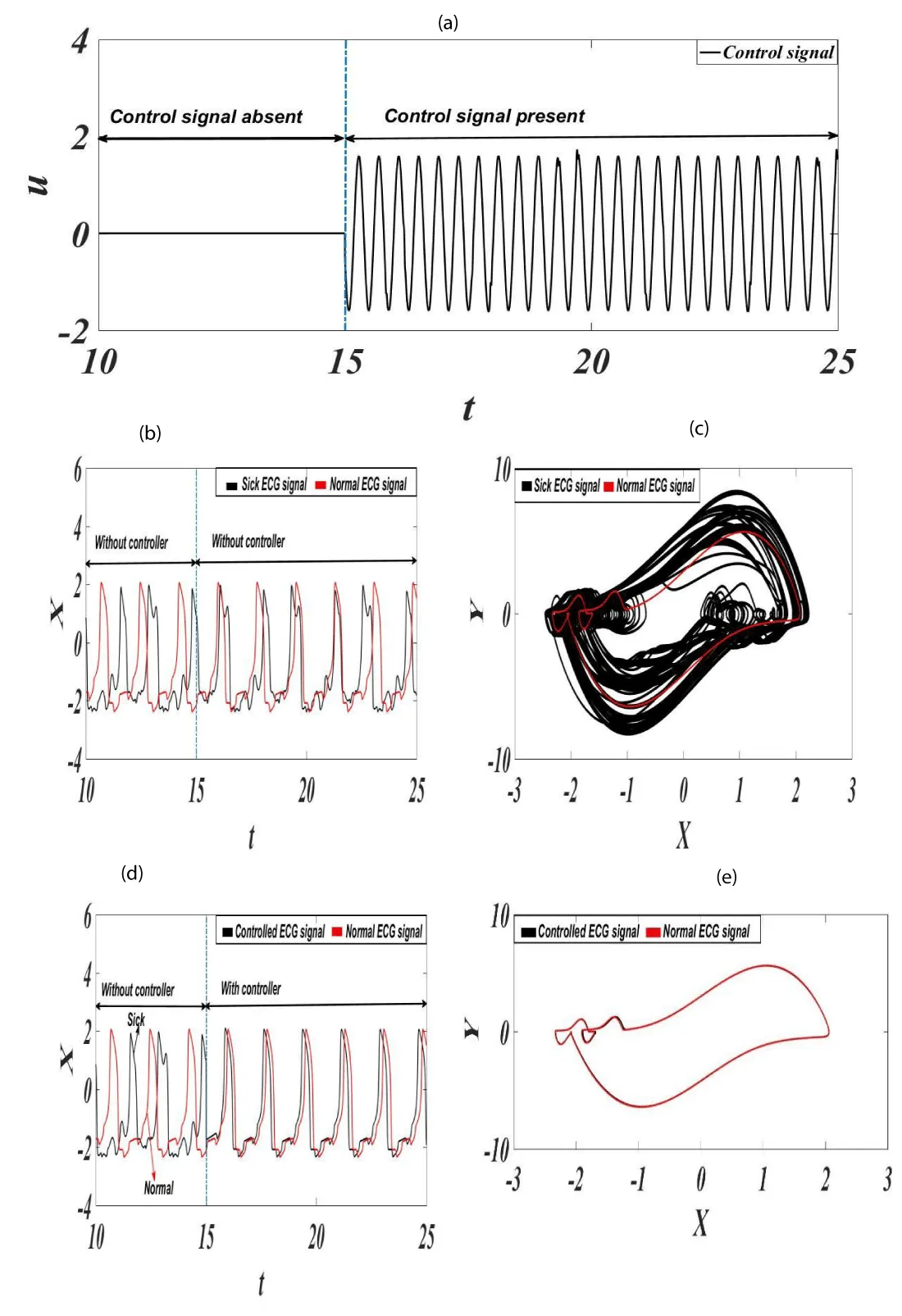
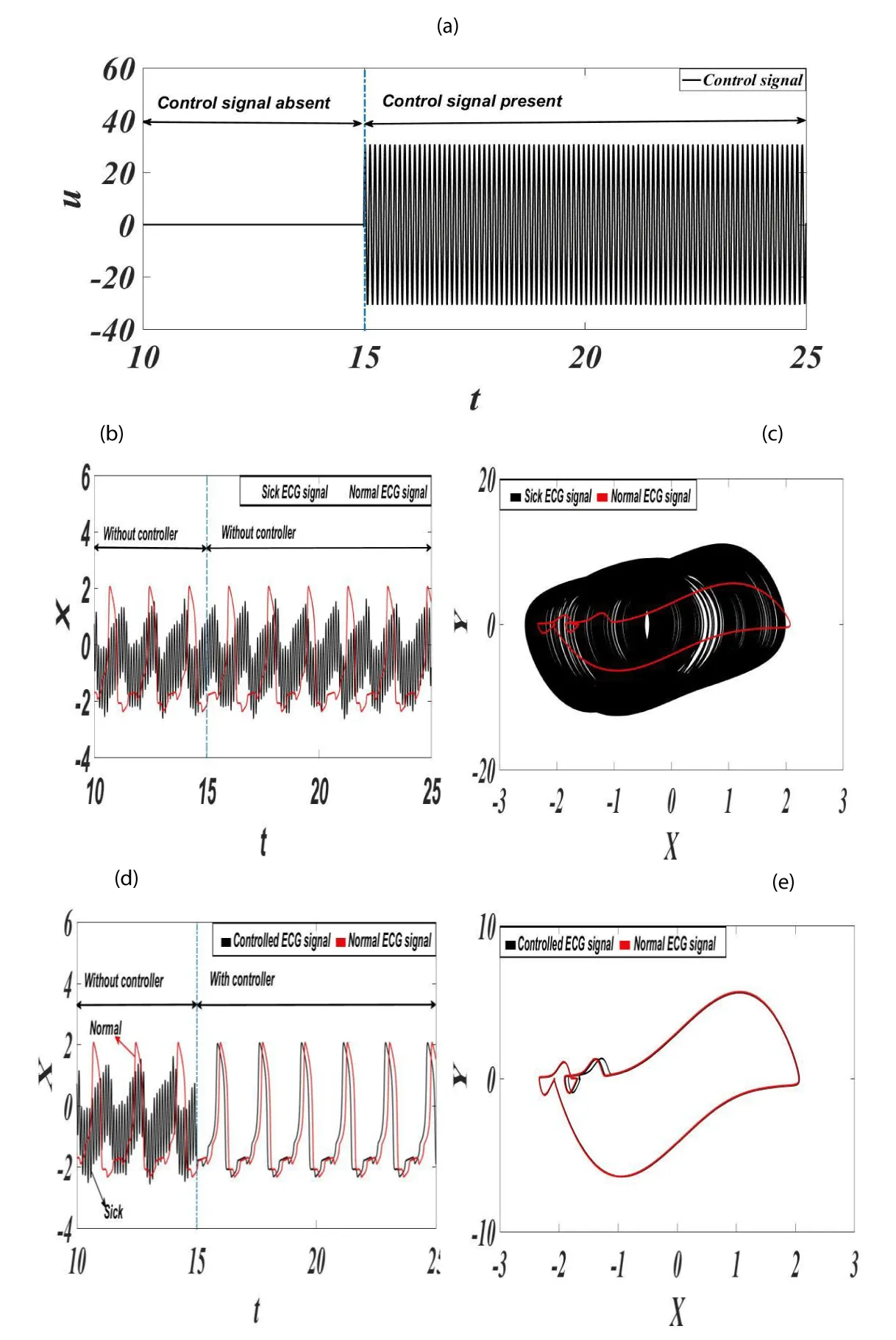
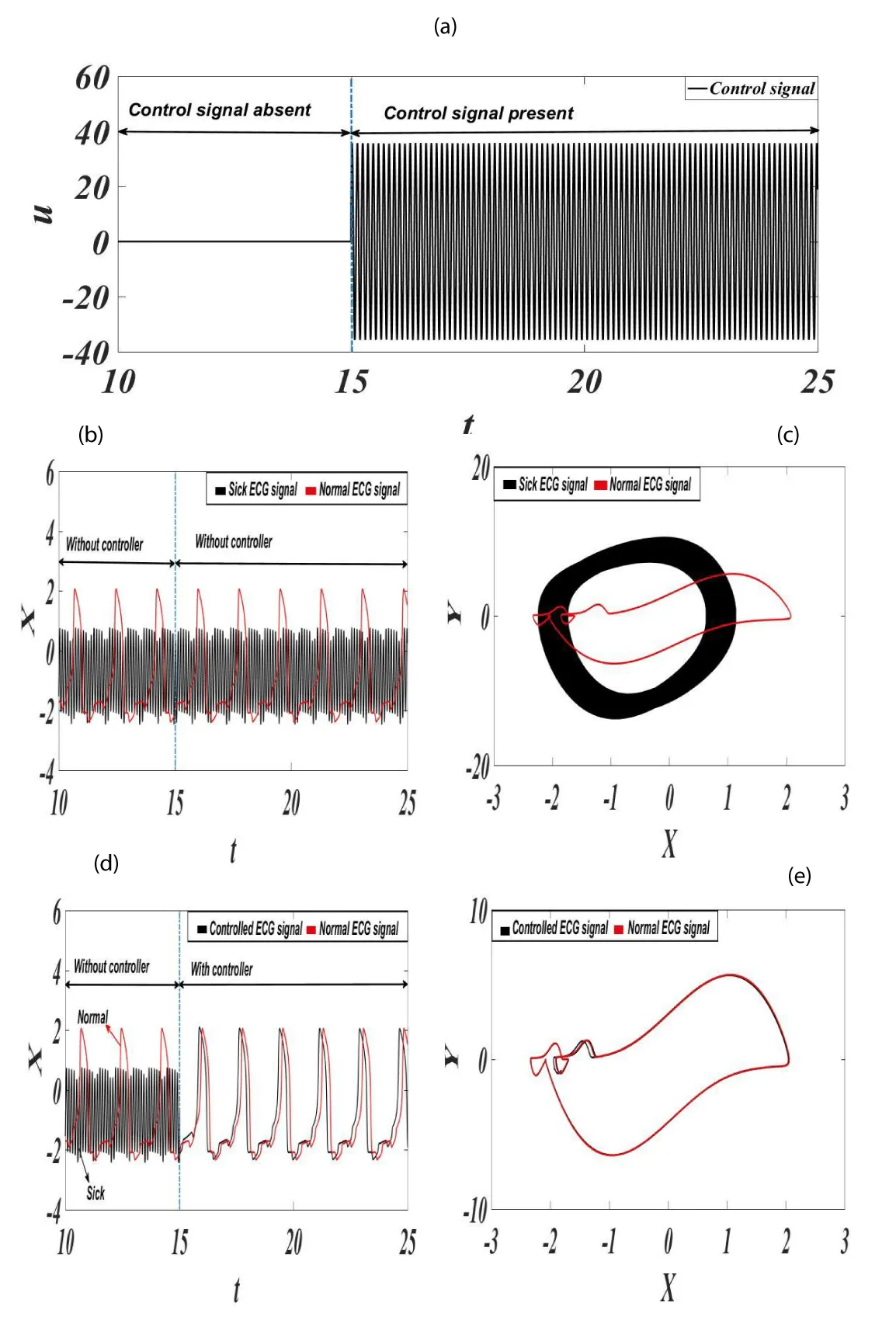
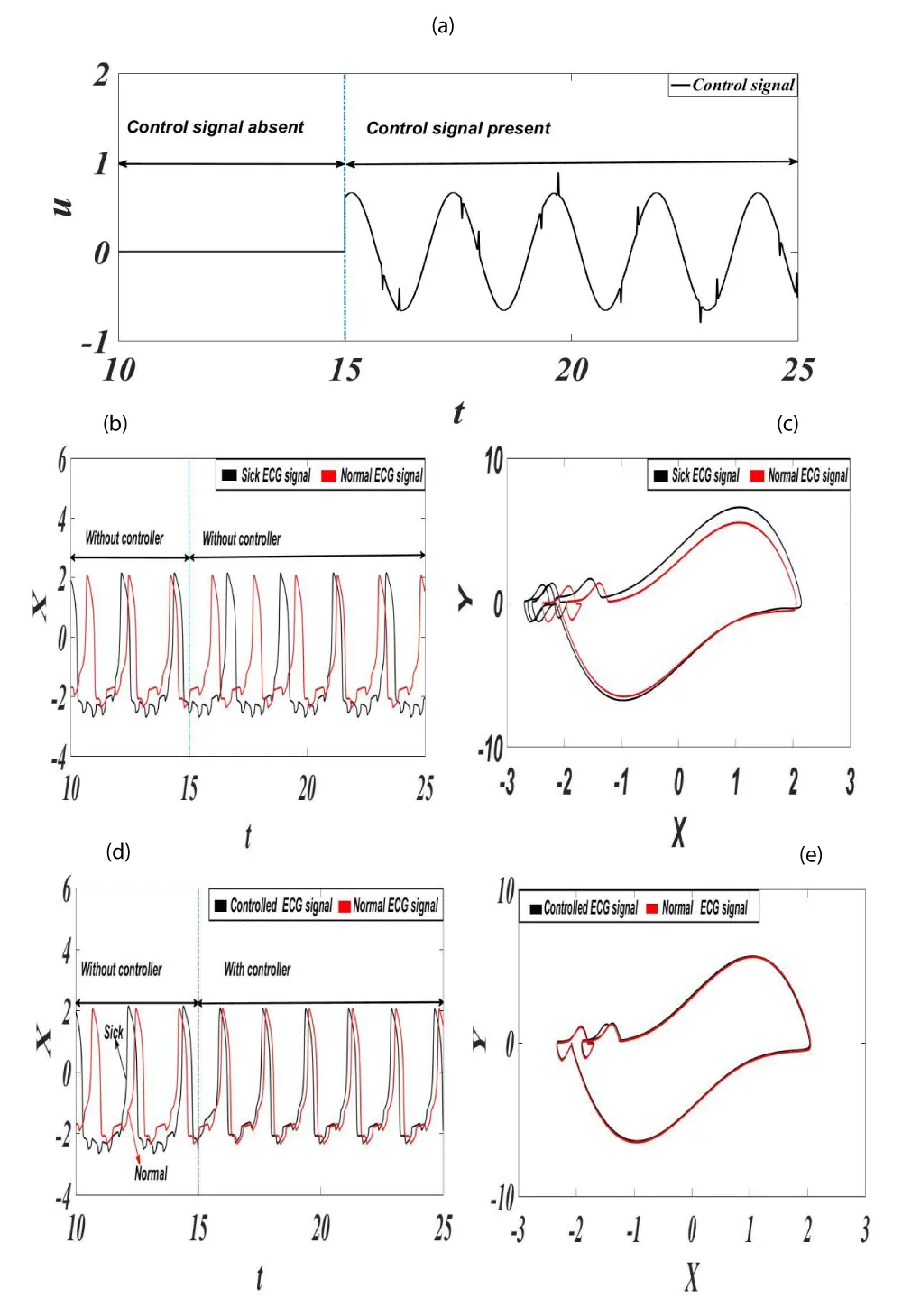
When the control signal u is applied to the system (1) in its sick state, the controlled ECG dynamics are shown in Figures 13-16 respectively. Figure 13 shows those obtained in the case of ventricular flutter. For ventricular fibrillation, they are shown in figure 14. Figure 15 shows the results for atrial fibrillation, and figure 16 for atrial flutter.
Figure 13: (a) Control signal. (b) Uncontrolled synthetic ECG time series. (c) Uncontrolled synthetic ECG state space. (d) Controller synthetic ECG time series. (e) Controller synthetic ECG state space.
Figure 14: Control signal. (b) Uncontrolled synthetic ECG time series. (c) Uncontrolled synthetic ECG state space. (d) Controller synthetic ECG time series. (e) Controller synthetic ECG state space.
Figure 15: Control signal. (b) Uncontrolled synthetic ECG time series. (c) Uncontrolled synthetic ECG state space. (d) Controller synthetic ECG time series. (e) Controller synthetic ECG state space.
Figure 16: Control signal. (b) Uncontrolled synthetic ECG time series. (c) Uncontrolled synthetic ECG state space. (d) Controller synthetic ECG time series. (e) Controller synthetic ECG state space.
Figure 16. Control signal. (b) Uncontrolled synthetic ECG time series. (c) Uncontrolled synthetic ECG state space. (d) Controller synthetic ECG time series. (e) Controller synthetic ECG state space Figures 13-16 show the action of the controller in cardiac arrhythmia situations. The synthetic ECGs show a qualitative and quantitative approximation between controlled and normal dynamics. Both the phase spaces and the time traces clearly show a very strong improvement in the performance of the highlighted control scheme, as well as its ability to replace a pathological cardiac rhythm with a normal one. The proposed intelligent control scheme shows its ability to make abnormal dynamics disappear.
It can be seen from the curves in figures 13-16 that the action of the controller starts at 15 s. Before 15 s, the controller has no effect on the heart. In the case of ventricular flutter, the control signal, once engaged, evolves at a frequency of 2.4 Hz. In ventricular fibrillation, the control signal has a frequency of 7.2 Hz. In atrial fibrillation, the control signal has a frequency of 8.2 Hz. In atrial flutter, a frequency of 0.6 Hz is observed. Whether in ventricular flutter, ventricular fibrillation, atrial fibrillation or atrial flutter, as observed in normal rhythm, the controlled dynamics clearly show the presence of the QRS complex and P and T waves. We also note the disappearance of the R and S peaks, reflecting the controller's skill in solving this problem
Thus, the feedback linearization control (FBL) method with the integration of an artificial neural network is very effective and robust for the control of pathological heartbeats.
Electronic implementation
In this subsection, we present the results obtained by electronic simulation using OrCAD-PSpice software. This is one of the most widely used simulations in electronic product design, whether for PCB design, IC design or other electrical systems. For the analysis of the most important electronic circuits, OrCAD-PSpice seems to be the most suitable simulation. Wired assemblies in this software allow the use of components with values that reproduce real components as effectively as possible. Once the device has been wired, the results can be analyzed in all their facets, using tools as varied as they are sophisticated. A large number of research studies have shown that OrCAD-PSpice is a world reference in the field of circuit design and simulation [4,27], as it possesses some of the most interesting features, including: the possibility of creating virtual components, using manufacturers' data sheets, downloading component libraries.
These include: reducing time wasted in choosing component values before the practical implementation of the system and exploring the advantages of different practical implementation options. Faced with the complexity of creating electronic assemblies whose results can be used to interpret real phenomena, OrCAD-PSpice software helps designers to solve problems at different levels of abstraction, to better understanding the interactions between the various components making up the system.
To implement the mathematical system on the OrCAD-Pspice software, Kirchhoff's and Ohm's laws are used and the system is modeled in the form of differential equations [27]. In this subsection, the dynamics of the system in its state of normal functioning are presented. The system used is the one described by the functional model in Figure 3.
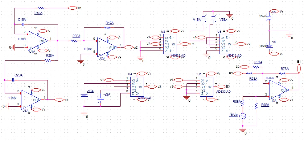
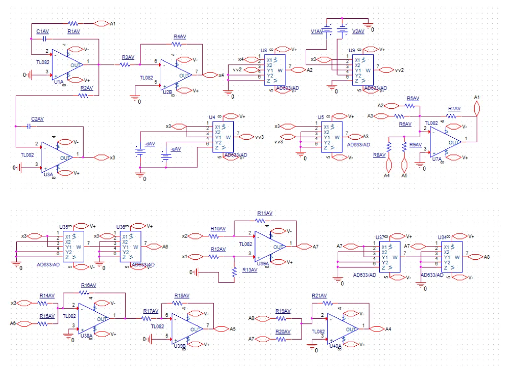
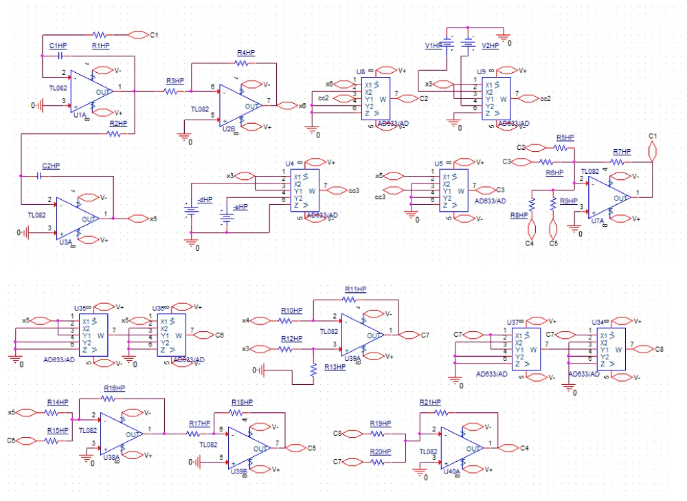
Using electronic equivalence techniques and operational amplifier integration (AOP) principles, the OrCAD-PSpice assembly of the SA oscillator, AV oscillator, and HP oscillator coupled together is shown in Figures 17-19 respectively.
Figure 17: Electronic equivalence of the circuit representing the SA oscillator mounted on OrCAD-PSpice software.
Figure 18: Electronic equivalence of the circuit representing the AV oscillator mounted on OrCAD-PSpice software.
Figure 19: Electronic equivalence of the circuit representing the HP oscillator mounted on OrCAD-PSpice software.
The above circuit implements the analog equivalence of the SA oscillator. It is composed of nine (9) resistors (
, and
), 2 capacitors (
and
), 4 operational amplifiers (TL082), 4 multipliers (AD633/AD), DC voltage sources to power integrated circuits (AOP and multipliers) for some and for others they are used as parameters of the equivalent circuit. We also note an AC power source (
) used to excite the circuit. Using the principle of Kirchhoff's laws to Ohm's law, the relationship between the inputs is given below:
From equation (35), we obtain equation (36) below.
The substitution of equations (31) and (33) in (35) gives us equation (37).
The relationships between the parameters of the SA node and the data in equation (37) allow us to establish the following correspondences given by equation (38).
Figure 18. Electronic equivalence of the circuit representing the AV oscillator mounted on OrCAD-PSpice software.
In this case (Figure 18), the analog equivalence is that of the AV oscillator. This figure shows 21 resistors (
, 2 capacitors
, 8 operational amplifiers (TL082), 8 multipliers (AD633/AD), DC voltage sources to power integrated circuits (AOP and multipliers) for some and others they are used as parameters of the equivalent circuit. The principle of Kirchhoff's laws to Ohm's law is used to establish the relationship between the inputs. The establishment of linear and cubic terms with delay is obtained using Taylor series expansion [68]. For a delayed variable
, where T is the delay, Taylor's series expansion allows it to be decomposed as follows:
So
and
Similar reasoning to the previous case (figure 16) gives us the following relationships:
By substituting equations (41), (43), (48) and (49) into (50), we obtain equation (51).
Starting from equation (50) and the SA oscillator equation (equation (1)), the relationships between the parameters are established by the correspondences given in equations (52), (53), and (54).
Figure 19. Electronic equivalence of the circuit representing the HP oscillator mounted on OrCAD-PSpice software.
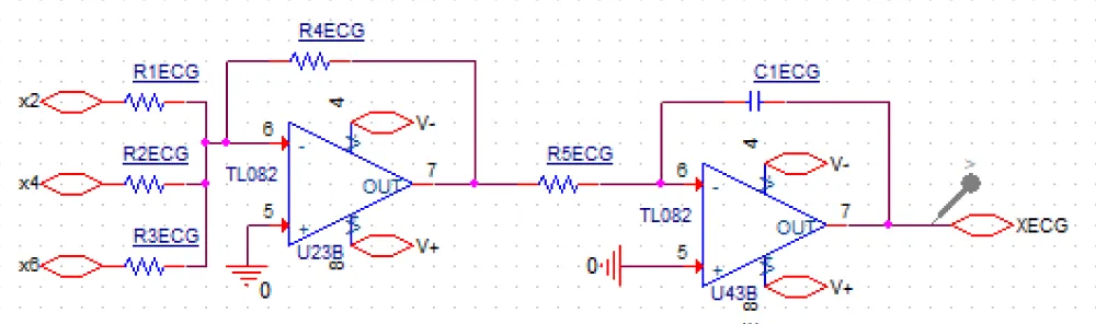
Figure 20: Electronic block for ECG signal generation mounted on OrCAD-PSpice software.
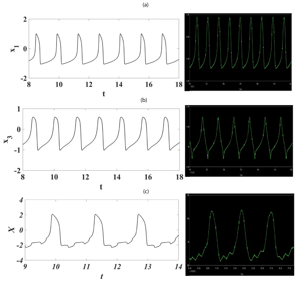
Figure 21: Curves obtained digitally and by electronic simulation with OrCAD-PSpice software: (a) case of SA oscillator; (b) case of AV oscillator; (c) case of ECG signal.
The analog equivalence for the HP oscillator is shown in Figure 18. This figure shows 21 resistors
, 2 capacitors
, 8 operational amplifiers (TL082), 8 multipliers (AD633/AD), DC voltage sources to power integrated circuits (AOP and multipliers) for some, and for others they are used as equivalent circuit parameters.
Using Kirchhoff's laws, Ohm's law, and Taylor's series expansion, an analogous analysis to the AV oscillator is used to obtain the following relationships:
The substitution in equation (65) of equations (56), (58), (63) and (64) gives the following equation (66).
Equivalences between the parameters of the HP oscillator (equation (1)) and those of equation (66) are given by equations (67), (68) and (69).
The block wired in the OrCAD-PSpice software to generate the ECG signal is shown in figure (20).
Note that AOPs with single-input feedback capacitors can be described as integrator modules, and for multi-input cases, they are called integrator-summer modules. Note that these modules can be used to sum the system's monomials. The change from a negative to a positive sign is made using unity-gain inverter modules with a feedback resistor.
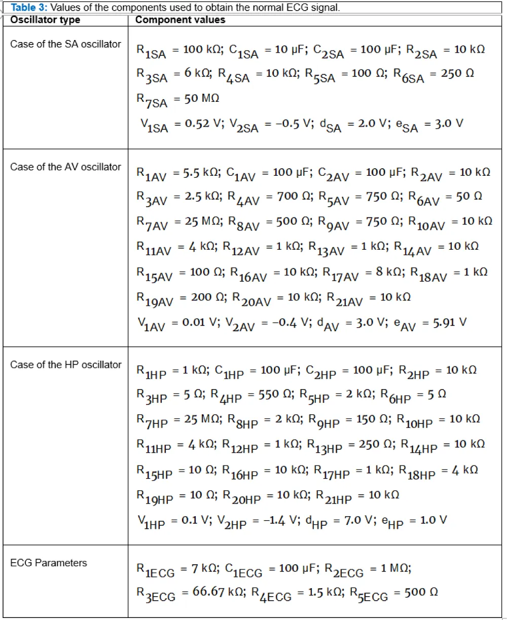
The values corresponding to each of the components used to generate the various signals are given in Table 3.
The curves presented are obtained for a simulation step size called maximum step size and given by Sc = 0.01s. The polarization voltages V + and V – are 15 V and – 15 respectively.
Considering the normal case
, Figure 21 compares some of the curves obtained by OrCAD-PSpice electronic simulation and digital simulation.
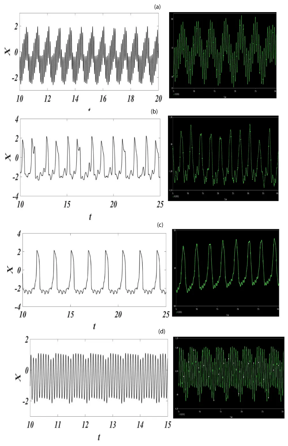
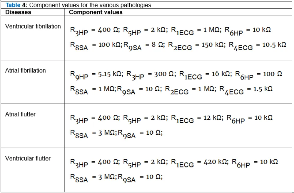
To obtain the diseased dynamics, the functional diagram given in figure 6 is considered. The curves obtained are shown in Figure 22. The basic values for obtaining the normal ECG given in Table 3 are maintained for some, and those modified according to the pathologies are given in Table 4. Note that the VSIN function represented by
is parameterized according to the data specific to each disease (VAMPL and FREQ).
Figure 22: Synthetic ECGs obtained digitally and by electronic simulation with OrCAD-PSpice software: (a) ventricular fibrillation; (b) atrial fibrillation; (c) atrial flutter; (d) ventricular flutter.
Conclusion
In this work, it was a question of implementing a controller on an electronic system generating pathological heart rhythms. In order to bring pathological rhythms as close as possible to normal rhythms, an intelligent control system based on feedback linearization (FBL) was implemented, incorporating an artificial neural network to compensate for the unknown dynamics. The variable considered was the ECG signal. ECGs were generated using a reduced-order mathematical model consisting of three nonlinear oscillators linked by delayed Duffing-type connections incorporating cubic nonlinear terms. The dynamics produced showed close agreement with experimental measurements. The controller was applied to the SA node to track the trajectory of its signals so that it follows the desired state. The learning rate representing the incorporation of artificial neural networks into a Lyapunov-based control scheme was taken to be non-zero (μ≠0), and adjusting the control parameter λ was used to improve the convergence of the closed-loop error. The results obtained show the effectiveness and robustness of the controller in avoiding the occurrence of a heart attack by approximating the ECG signal to the expected normal behavior. To demonstrate that the proposed heart model can derived from mathematical modeling, an electronic simulation using analog components has been carried out using OrCAD-Pspice software. The results obtained show good agreement with the numerical simulations.
Declarations
Funding statement: This research did not receive any specifi grant from funding agencies in the public, commercial, or not-for-profi sectors.
Data availability statement: No data was used for the research described in the article.
Declaration of interest_s statement: The authors declare no competing interests.
Additional information: No additional information is available for this paper.
Appendix



 Save to Mendeley